In statistics, Markov chain Monte Carlo (MCMC) methods (which include random walk Monte Carlo methods) are a class of algorithms for sampling from probability distributions based on constructing a Markov chain that has the desired distribution as its equilibrium distribution. The state of the chain after a large number of steps is then used as a sample of the desired distribution. The quality of the sample improves as a function of the number of steps.
Usually it is not hard to construct a Markov chain with the desired properties. The more difficult problem is to determine how many steps are needed to converge to the stationary distribution within an acceptable error. A good chain will have rapid mixing—the stationary distribution is reached quickly starting from an arbitrary position—described further under Markov chain mixing time.
Summary
Monte Carlo method의 단점은 주어진 density function p(x)로부터의 random number generation이 쉽지 않으면 효용도가 떨어진다는 점이다.
MCMC는 이러한 Monte Carlo method의 단점을 보완한 방법으로 density function p(x)로부터 직접 random number generation 하는 대신에 stationary distribution p(x)의 Markov chain을 만들어 random number generation 하는 것이다.
- Step #1
Stationary distribution p(x)을 따르는 Markov chain {X0, X1, ..., Xt}를 만든 후 Xt를 저장한다.
(Xt는 t시간에서의 state vector이다.) - Step #2
Step #1을 n번 반복 후 저장된 n개의 Xt들이 density function p(x)를 따르는 random numbers이다.
좋은 random number generation을 위해서는 step #1에서 t를 충분히 크게 해 주어야 하고, 이 과정은 초기값에 영향을 받지 않게 하는 과정으로 burn-in이라고 부른다.
여기서 Markov chain을 생성하는 알고리즘이 Metropolis-Hastings algorithm이다.
Lectures
Lecturer: Professor Daphne Koller - Stanford Univ.
Other Sources
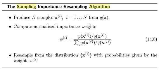
As we explore the state space, we can also construct samples as we go along in such a way that the samples are likely to come from the most probable parts of the state space.
pseudo-random numbers
linear congruential relation
![]()
![]() seed
seed
Mersenne Twister 실제로 쓰이고 있는 랜덤넘버생성 알고리즘
하지만 모두 리얼 랜덤 넘버는 아니다.
랜덤 넘버인지 테스트하는 방법 entropy:
랜덤 시퀀스 일수록 redundancy가 작고, 압축하기가 어렵다.
Mersenne Twister는 uniform distribution의 알고리즘을 생성하는데 다른 분포의 랜덤 넘버를 생성하고 싶을 수도 있다. -> Gaussian 분포같은거.
The Box-Muller scheme
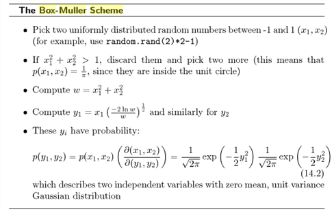
rejection이라는 개념 때문에 Box-Muller Schem이 중요하다.
처음 생성된 두 개의 랜덤 넘버가 원안에 들어오지 않을 때 그 샘플은 reject된다.
이 것을 이용해서 원하는 형태의 넘버를 빠르게 생성할 수 있다!(운이 좋으면)
Monte Carlo or Bust
Monte Carlo 원리
어떤 iid분포에서 샘플을 많이 뽑을수록, 그 샘플의 분포는 그 실제 분포와 가까워짐
![]()
![]()
The Proposal Distribution
이제 ![]() 만 샘플링하기 쉽다면 문제가 없다. 하지만 보통
만 샘플링하기 쉽다면 문제가 없다. 하지만 보통 ![]() 는 샘플링하기 어렵다.
는 샘플링하기 어렵다.
![]() 는 계산하기는 쉽지만 샘플링하기는 어렵다.
는 계산하기는 쉽지만 샘플링하기는 어렵다.
대신 샘플링하기 쉬운 ![]() 를 만듦으로써 문제를 풀 수 있다.
를 만듦으로써 문제를 풀 수 있다.
![]() 로 샘플링하고
로 샘플링하고 ![]() 의 계산과 비교해서 많이 차이나면 reject하는 것이다.
의 계산과 비교해서 많이 차이나면 reject하는 것이다.
![]() 는 계산하기는 쉽지만 샘플링하기는 어렵다는 가정이 말이 안되는 것은 아니다. 이런 경우는 흔하다. Gaussian 분포 같은 경우도 분포의 함수가 있어 계산하기 쉽지만 샘플링하는 것은 간단하지 않다.
는 계산하기는 쉽지만 샘플링하기는 어렵다는 가정이 말이 안되는 것은 아니다. 이런 경우는 흔하다. Gaussian 분포 같은 경우도 분포의 함수가 있어 계산하기 쉽지만 샘플링하는 것은 간단하지 않다.
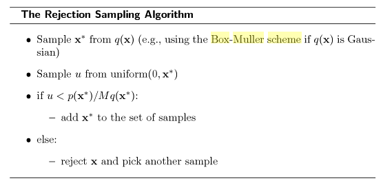
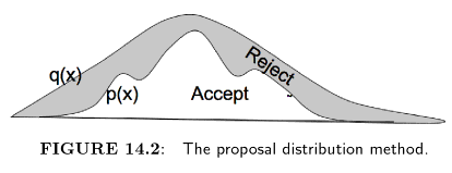
M이 클수록 reject를 많이 하게 된다.
![]() 3
3
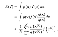
 는 그 함수의 중요함을 표현하는 weight로 작용한다.
즉 actual 분포 ![]() 와
와 ![]() 가 비슷할수록 중요하게 된다.
가 비슷할수록 중요하게 된다.
Markov Chain Monte Carlo
The link to sampling that we need is that if the transition probabilities reflect the distribution that we wish to sample from, then a random walk will explore that distribution.
전이 확률이 우리가 샘플링하고 싶은 분포를 반영하고 있다면, 랜덤웍은 그 분포를 탐험할 것이다.
하지만 랜덤워크는 왔다갔다하므로 매우 비효율적이다.
우리의 마코프체인을 만들어서 해결
ergodicity: Markov Chain의 state의 network가 connected 되어 있다.
aperiodic: acyclic network이다.
![]()

위에가 성립할려면 reversible해야 한다. 즉
![]() detailed balance condition. then,
detailed balance condition. then,
this is known as the detailed balance condition and the fact that it leaves the distribution ![]() alone is fairly obvious with a little calculation.???
alone is fairly obvious with a little calculation.???
Markov Chain이 detailed balance condition을 만족하면, ergodic하다 그러므로 ![]() 이고 다음이 성립한다.
이고 다음이 성립한다.
 =
=![]()
T는 분포 p를 변화시키지 못한다는 뜻이다.
detailed balance condition를 만족하는 Markov Chain을 생성할 수 있다면, 그 마코프 체인은 우리가 샘플링하고 하는 ![]() 에 변화를 주지 않기 때문에 그 Markov Chain을 이용해서
에 변화를 주지 않기 때문에 그 Markov Chain을 이용해서 ![]() 를 샘플링 할 수 있다.
를 샘플링 할 수 있다.
우리가 샘플링 할 수 있는 ![]() 를 갖고 있다고 가정
를 갖고 있다고 가정
![]() 가 위에서의 전이확률
가 위에서의 전이확률 ![]() 이다.
이다.
Mertoplos-Hastings 은 rejecting sampling이랑 개념이 비슷하다.
원하는 샘플만 keep한다.
하지만 rejecting sampling이랑 달리 현재 샘플 하나를 rejecting했다면, 다른 sample 을 pick하기 보다는, 단순히 전에 accepted된 sample의 copy한다.
sample이 keep될 확률은 다음과 같다.
![]()
![]() 에서 보듯이
에서 보듯이 ![]() 가 detailed balance condition를 만족할수록 식이1에 가까워진다. 즉 accept될 확률이 커진다.
가 detailed balance condition를 만족할수록 식이1에 가까워진다. 즉 accept될 확률이 커진다.
분모 분자가 ![]() 와
와 ![]() 가 바뀌네 reversible한 성질과 관계가 있을 것 같은데;
가 바뀌네 reversible한 성질과 관계가 있을 것 같은데;
왜 이 알고리즘이 동작하는가?
각 스텝은 q에서 샘플된 현재 값 ![]() 를 사용한다.
를 사용한다.
마코프 체인이 좀 더 바람직한 state(원래분포에 가까운 샘플)에 근접하면 accept
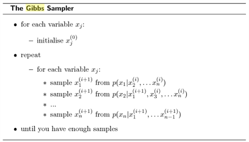
Gibbs Sampling
Metropolis-Hasting Algorithm의 다른 변형은 full conditional probability ![]() 을 아는 것에서 시작한다. 편의를 위해
을 아는 것에서 시작한다. 편의를 위해
![]() 라고 표시한다.
라고 표시한다.
우리는 다음과 같은 네트워크로부터의 확률의 집합을 다루게 될 것이다.
![]()
![]() 을 알고 있다면,
을 알고 있다면,
아마도 그것을 다음과 같이 proposal 분포로 사용해야 할 것이다.
![]()
그 다음 Metroplis-Hastings을 사용한다면 다음과 같은 acceptance probability ![]() 가 나온다.
가 나온다.
![]()
![]()
![]()
![]()
![]() ,
, ![]() 이므로
이므로
아 수식 뭔가 이상한 것 같고, 결국 결론은 항상 ![]() 이 되어서 항상 acceptance한다.
이 되어서 항상 acceptance한다.
Bayesian Network
Network의 cycle이 없어야 한다.
DAGs(directed, acyclic graphs)라고 부른다.
Conditional probability tables로 표현했다면 Bayesian networks라 부른다.
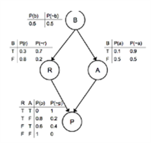
예제: Exam Panic
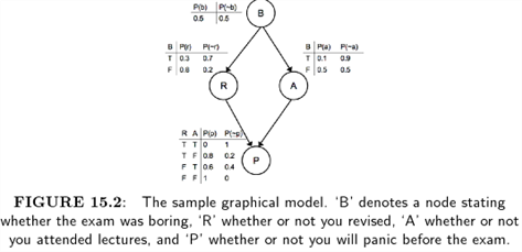
B : Boring
A : Attend lectures
R : revise
P : panic
you panicking
If we have a set of observations that can be used to predict an unknown outcome, then we are doing top-down inference or prediction, whereas if the outcome is known, but cause s are hidden, then we are doing bottom up inference or diagnosis.
Either way, we are working out the values of the hidden nodes given information about the observed nodes.
For example in Figure 15.2 we will start by predicting whether or not you will panic before exam, so it is the outcome that is hidden.
//
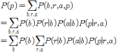
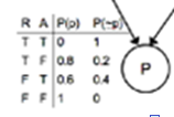
In order to compute the probability of panicking, we need to compute P(b,r,a,p), where the lower-case letters indicate particular values that the upper-case variables can take.
The wonderful thing about the graphical model is that we can read the conditional probabilities from the graph-if there is no direct link, then variables are conditionally independent given a node that is already included, so those variables are not needed.
For this reason, the computation we need for Figure 15.2 is
 (15.1)
If we know particular values for the three observable nodes, then we can plug them in and work out the probability.
In fact, the conditional independence gives us even more: if I know both whether or not you attended lectures and whether or not you revised, then I don't need to know if the course was boring, since there is no direct connection between 'B' and 'P'.
suppose that you didn't attend lectures, but did revise.
In that case, the probability of you panicking can be read off the final distribution table as 0.8
The power of the graphical model is when you don't have full information.
It is possible to marginalize over any of those variables by summing up the values.
So suppose that you know that the course was boring, and want to work out how likely it is that you will panic before the exam.
In that case you need to sum up the probabilities in Equation (15.1)
![]()
P(p)=P(b){P(r|b)P(a|b)P(p|r,a)+P(r|b)P(~a|b)P(p|r,~a)+P(~r|b)P(a|b)P(p|~r,a)+P(~r|b)P(~a|b)P(p|~r,~a)}
+P(~b){you can do it yourself}
=0.5x(0.3x0.1x0+0.3x0.9x0.8+0.7x0.1x0.6+0.7x0.9x1)
+0.5x(0.8x0.5x0+0.8x0.5x0.8+0.2x0.5x0.6+0.2x0.5x1)
= 0.684
The backward inference, or diagnosis, can also be useful.
Suppose that I see you panicking outside the exam.
You look vaguely familiar, but I'm not sure whether or not you came to the lecture.
I might want to work out why you are panicking-was it because you didn't come to the lectures, or because you didn't revise?
To perform this calculation I need to use Bayes's rule to turn the conditional prob around, just as was done for the Bayes' classifier.
So the computations that I need are:
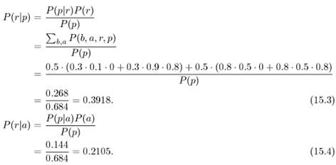
This use of Bayes' rule is the reason why this type of graphical model is known as a Bayesian network.
Even in this very simple example, the inference was not trivial, since there were a lot of calculations to do.
However, the problem if actually rather worse than that.
The computational cost of the simple algorithm we used is O(2n) for a graph with N nodes where each node can be either true or false.
In general the problem of exact inference on BN is NP-hard
However, for so-called polytree where there is at most one path between any two nodes,
the computational cost is much smaller-linear in the size of the network.
Unfortunately, it is rare to find such polytree in real examples, so we can either try to turn other networks into polytrees, or consider only approximate inference, which is the most common solution to the problem, and the method that we'll consider next.
We can speed things up a little by getting things into the form of Equation (15.1), where the summations were carefully placed as far to the right as possible, so that program loops can be minimised
By doing this the algorithm is as efficient as possible, but it is still NP-hard.
This is sometimes known as the variable elimination alg, which is a variation on the bucket elimination alg.
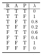
The idea is to convert the conditional prob table into what are called ![]() tables, which simply list all of the possible values for all variables, and which initially contain the conditional prob.
tables, which simply list all of the possible values for all variables, and which initially contain the conditional prob.
For example, the ![]() table for the P variable in Figure 15.2 is:
table for the P variable in Figure 15.2 is:
 <--
<--
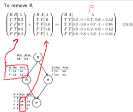
If I see you panicking outside the exam (so that P is true), then I can eliminate it from the graph by removing from each table all rows that have P false in them, and deleting the P column.
This simplifies things a little, but I have to do rather more in order to compute the prob of you having attended lectures.
I don't know whether you revised or not, and I don't know if you found the lectures boring, so I have to marginalise over these variables.
The order in which we marginalize doesn't change the correctness so we'll pick R first.
To eliminate it from the graph, we have to find all of the ![]() tables that contain it(there will be two of them containing R: the one for R itself and the one that we have just modified to remove P//아래그림의 빨간색)
tables that contain it(there will be two of them containing R: the one for R itself and the one that we have just modified to remove P//아래그림의 빨간색)
To remove R, we have to add together the products of the ![]() values that corresspond to places where the other values match ???행렬곱셈하는 것처럼
values that corresspond to places where the other values match ???행렬곱셈하는 것처럼
So to complete the entry where B is true and A is false, we have to multiply together the values where B, A, R are respectively true, false, true in the two tables and then add to that the product of where B, A, R are respectively true, false, false. ???
We can do the same thing in order to eliminate B, which involves all three of the tables, and this will enable the computation of the conditional prob of you attending lectures given that I saw you panicking before the exam.
15.1.2 Approximate Inference
Since the variable elimination algorithm will only take you so far, for reasonably sized BN there is no choice but to perform approximate inference.
There is no choice[alternative] but to do so. (출처: 동아 프라임 한영사전)
그렇게 할 수밖에 없다
MCMC
The basic idea of using MCMC methods in BN is to sample from the hidden variables, and then weight the samples by their likelihoods.???
Creating the samples is very easy: for prediction, we start at the top of the graph and sample from each of the known prob dist
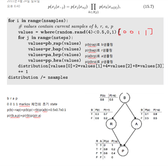
Using Figure 15.2 again, we generate a sample from P(b) and then use that value in the cond prob tables for R and A to compute P(r|b=sample value) and P(a|b=sample value).
These three values are then used to sample from P(p|b,a,r).
We can take as many samples as we like in this way, and expect that as the number of samples gets large, so the frequency of specific samples will converge to their expected values.
In this sampling method, we have to work through the graph from top to bottom and select rows from the cond prob table that match the previous case.
This is not what we would do if we were constructing the table by hand ???
suppose that you wanted to know how many courses you did not attend the lectures for because the course was boring.
You would simply look back through your courses and count the # of boring courses where you didn't go to lecture, ignoring all the interesting courses.
We can use exactly this idea if we use rejecting sampling
The method samples from the unconditional distribution and simply rejects any samples that don't have the correct prior prob???
It means that we can sample from each distribution independently, and then throw away any samples that don't match the other variables.???
This is obviously computationally easier, but we might have to reject a lot of sample.
The solution to this problem is to work out what evidence we already have and use this evidence to assign likelihoods to the other variables that are sampled.
Suppose that we sample from P(b) and get value 'true'.
If we already know that we did revise, then we weight the observation P(r|b) by the appropriate probability, which is 0.3

We continue through the other probability if we do have evidence.
However, we can do rather better than this by using the full MCMC framework.
We start by setting values for all of the possible probabilities, based on either evidence or random choices.
This gives us an initial state for a Markov chain.
Now Gibbs sampling will find us the maxima of our probability distribution given enough samples.
The probability in the network are:
![]()
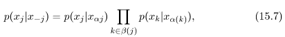
![]()
![]()
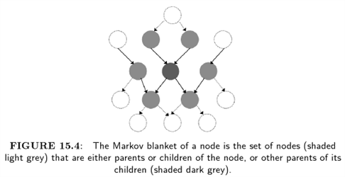
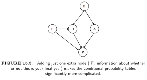
For any node we only need to consider its parents, its children, and the other parents of the children, as shown in Figure 15.4.
This set is known as the Marknov blanket of a node.
Given these calculations, computing the inference on any real BN generally consist of using Gibbs sampling in order to approximate the inference.
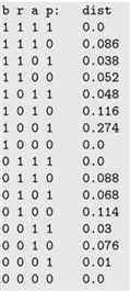
For the exam panic example, the alg to perform the Gibbs sampling consist of computing the probability distributions (possibly by using parts of the variable elimination algorithm)
and then sampling from it:
전체적인 흐름을 보자면, 조건부 확률 테이블이 주어졌을 때 예제처럼 P(p)이런 것을 계산하는 것이 NP-hard 의 계산시간이 걸리기 때문에, 샘플링 기법으로 근사하는 것이 목적이다.
15.1.3 Making Bayesian Networks
If we are given the structure and CPT of the BN, we can perform inference on it by using Gibbs sampling or, if the network is simply enough, exactly.
However, this raises the important question about where the BN itself comes from.
Unfortunately, the news in this area isn't particularly good: the computational costs of searching over trees are immense, as we shall see.
It is not uncommon for people to create the entire network by hand, and only then to use algorithms in order to perform inference on the network.
Constructing BN by is obviously very boring to do, and unless it is based on real data then it is subjective: putting a whole lot of effort into inference is a waste of time if the data you are inferring about bears no resemblance to reality ???
So why is it so difficult to construct BN?
First, we have already seen that the problem of exact inference on BN was NP-hard, which is why we had to use approximate inference.
Now let's think about the structure of the graph a little.
If there are N nodes(N random variables in the graph), then how many different graphs are there?
For just three nodes(A,B,C) we can leave the three unconnected, connect A to B and leave C alone, connect B to A and leave C alone
For ten nodes there are O(1018) possible graph, so we are not going to be searching oveer all of them. Further, we might want our algorithm to be thing to include latent variables, that is, hidden nodes, which might be a sensible thing to do in terms of explaining the data, but it does make the problem of search even worse.
We've talked about search before: So can we use those methods to solve this problem?
Yes once we have worked out an objective function to maximize.
We want to reward graphs that explain the data well, but we also want to appeal to Occam's razor to ensure that the graphs are as simple as possible.
Typical methods are to use an on objective function based on the MDL or related information-theoretic measures.
Then hill climbing or similar algorithms are used to perform local search around a set of random starting graphs.
You might be wondering why it is not possible to use a genetic algorithm.
It is, but given # of iterations of the GA, each of which would involve constructing hundreds of possible networks, testing them by performing inference, and then combining them, the computational expense rules it out as a practical possibility.
As it is such an important problem, there has been a lot of very advanced work on it
Given that we cannot make the entire graph, we will consider the compromise situation, where we try to compute the CPT for a known graph based on data.
This is quite a sensible compromise: you assume that some expert can put together a network that shows how variables relate to each other, effectively a 'catoon' of the data generating process, and then you use data in order to compute the CPTs.
However, it is still difficult.
The idea is to choose the PD to maximize the likelihood of the training data.
If there are no hidden nodes, then it is possible to compute the likelihood directly:
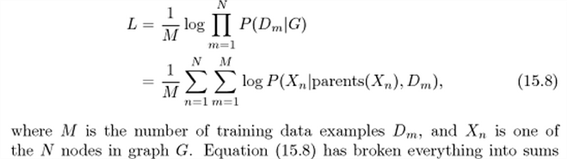
over each node individually, which means that we can compute each separate conditional probability table.
To compute the values of the table, you just need to count how often you have panicked in an exam given each of the possible values for having revised and attended lectures, and normalize it to make it into probability.
The danger with this is that with small amounts of data there could be examples that have not happened in training, and that will therefore have prob 0, although this can be dealt with by including proir probablities and using Bayes's rule to update the estimates using the real data.
Obviously, this doesn't work if there are hidden nodes, since we don't know values for them in the data.
Surprisingly, getting around this problem isn't as difficult as might be expected.
The key is to see that if we did have values for them, then Eq(15.8) could be used.
We can estimate values for them by inference followed by a maximisation step, making this as EM alg
15.2 Markov Random Fields
BN are inherently asymmetric, since each edge had an arrow on it.
If we remove this constraint, then there is no longer any idea of children and parent nodes.
I also makes the idea of conditional independence that we saw for the BN easier: two nodes in a Markov Random Field are conditionally independent of each other, given a third node, if there is no path between the two nodes that doesn't pass through the third node.
This is actually a variation on the Markov property, which is how the networks got their name: the state of a particular node is a function only of the states of its immediate neighbours, since all other nodes are conditionally independent given its neighbours.
You might think that this fact would make inference on MRFs simpler, but unfortunately it doesn't; in general it is still a #P-hard problem.
However, there are particular applications where MRF methods have turned out to be particularly useful, often for image.
The original theory of MRF's was worked out by physicists, initially by looking at the Ising model, which is a statistic description of a set of atoms connected in a chain, where each can spin up (+1) or down (-1) and whose spin affects those connected to it in the chain. Physicists tend to think of the energy of such systems, and argue that stable states are those with the lowerst energy, since the system needs to get extra if it wants to move out of this state.
For this reason, the jargon of MRFs is in terms of energies, and we therefore want the energy of our pair of images to be low when the pixels match, higher when they do not.
So we write the energy of the same pixel in two images as ![]() , where
, where ![]() is a positive constant.
is a positive constant.
Note that if the two pixels have the same sign then the energy is negative, while if they have opposite signs then the energy is positive and therefore larger.
The energy of two neighbouring pixels is ![]() and we can just add these components together to get the total energy:
and we can just add these components together to get the total energy:
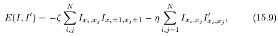
![]() 이미지가 일치하면 +1이라서 에너지가 -가 됨
이미지가 일치하면 +1이라서 에너지가 -가 됨
There is now a simple iterative update algorithm, which is to start with noisy image I and ideal I', and update I so that at each step the energy calculation is lower.
So you pick one pixel ![]() for some values of
for some values of ![]() at a time and compute the energies with this pixel being set to -1 and 1, picking the lower one.
at a time and compute the energies with this pixel being set to -1 and 1, picking the lower one.
In probabilistic terms, we are making the probability p(I,I') higher.
The algorithm then moves on to another pixel, either choosing a random pixel at each step or moving through them in some pre-determined order, running through the set of pixels until their values stop changing.
References
- http://en.wikipedia.org/wiki/Markov_Chain_Monte_Carlo
- http://sens.tistory.com/235
- http://web.archive.org/web/20110809043420/http://www.bioss.ac.uk/students/alexm/MCMCintroPresentation.pdf
- http://blog.naver.com/rupy400/130107459580
- http://videolectures.net/mlss09uk_murray_mcmc/
 Introduction to Markov Chain Monte Carlo & Gibbs Sampling (Cornell).pdf
- Markov Chain Monte Carlo (including implementation with R).pdf
- Markov Chain Monte Carlo Methods.pdf
- MCMC (Penn State).pdf
- MCMC Methods - Gibbs Sampling and the Metropolis-Hastings Algorithm.pdf
- Sampling Tutorial (USC).pdf
- [Paper] The Markov Chain Monte Carlo Revolution - Persi Diaconis - Stanford University
- http://ko.wikipedia.org/wiki/%EB%A7%88%EB%A5%B4%EC%BD%94%ED%94%84_%EC%97%B0%EC%87%84_%EB%AA%AC%ED%85%8C%EC%B9%B4%EB%A5%BC%EB%A1%9C_%EB%B0%A9%EB%B2%95
- Markov Chain Monte Carlo로 암호 해독하기
- 죄수들이 주고 받은 암호문 해독하기
- MCMC 개관
- http://jyeun426.tistory.com/18
- Sampling & MCMC
- Markov Chain Monte Carlo (MCMC) and Gibbs Sampling example(MATLAB)
- MC sample, MCMC, Gibbs Sampler, Metropolis